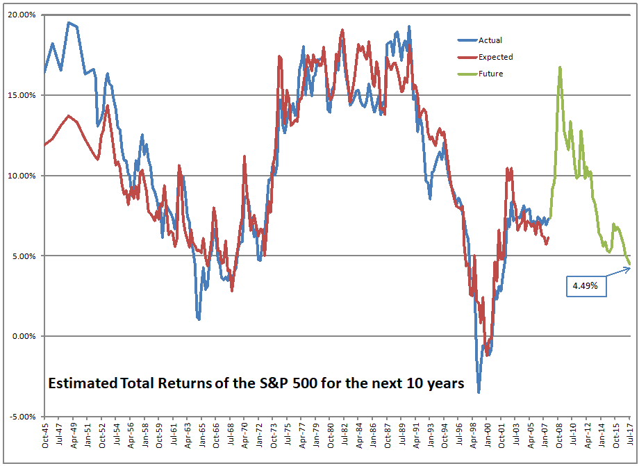
Another quarter goes by, the market rises further, and the the 10-year forward return falls again.? Here are the last eight values:?6.10%, 6.74%, 6.30%, 6.01%, 5.02%, 4.79%, and 4.30%, 3.99%. ?At the end of September 2017, the figure would have been 4.49%, but the rally since the end of the quarter shaves future returns down to 3.99%.
At the end of June the figure was 4.58%.? Subtract 29 basis points for the total return, and add back 12 basis points for mean reversion, and that would leave us at 4.41%.? The result for September month-end was 4.49%, so the re-estimation of the model added 8 basis points to 10-year forward returns.
Let me explain the adjustment calculations.? In-between quarterly readings, price movements shave future returns the same as a ten-year zero coupon bond.? Thus, a +2.9% move in the total return shaves roughly 29 basis points off future returns. (Dividing by 10 is close enough for government work, but I use a geometric calculation.)
The mean-reversion calculation is a little more complex.? I use a 10-year horizon because that is the horizon the fits the data best.? It is also the one I used before I tested it.? Accidents happen.? Though I haven’t talked about it before, this model could be used to provide shorter-run estimates of the market as well — but the error bounds around the shorter estimates would be big enough to make the model useless. It is enough to remember that when a market is at high valuations that corrections can’t be predicted as to time of occurrence, but when the retreat happens, it will be calamitous, and not orderly.
Beyond 10-years, though, the model has no opinion.? It is as if it says, past mean returns will occur.? So, if we have an expectation of a 4.58% returns, we have one 4.58%/yr quarter drop of at the end of the quarter, and a 9.5% quarter added on at the end of the 10-year period. That changes the quarterly average return up by 4.92%/40, or 12.3 basis points.? That is the mean reversion effect.
Going Forward
Thus, expected inflation-unadjusted returns on the S&P 500 are roughly 3.99% over the next ten years.? That’s not a lot of compensation for risk versus investment-grade bonds.? We are at the 94th percentile of valuations.
Now could we go higher?? Sure, the momentum is with us, and the volatility trade reinforces the rise for now.? Bitcoin is an example that shows that there is too much excess cash sloshing around to push up the prices of assets generally, and especially those with no intrinsic value, like Bitcoin and other cryptocurrencies.
Beyond that, there are not a lot of glaring factors pushing speculation, leaving aside futile government efforts to stimulate an already over-leveraged economy.? It’s not as if consumer or producer behavior is perfectly clean, but the US Government is the most profligate actor of all.
And so I say, keep the rally hats on.? I will be looking to hedge around an S&P 500 level of 2900 at present.? I will be watching the FOMC, as they may try to invert the yield curve again, and crash things.? They never learn… far better to stop and wait than make things happen too fast.? But they are omnipotent fools.? Maybe Powell will show some non-economist intelligence and wait once the yield curve gets to a small positive slope.
Who can tell?? ?Well, let’s see how this grand experiment goes as Baby Boomers arrive at the stock market too late to save for retirement, but just in time to put in the top of the equity market.? Though I am waiting until S&P 2900 to hedge, I am still carrying 19% cash in my equity portfolios, so I am bearish here except in the short-run.
PS — think of it this way: it should not have gone this high, therefore it could go higher still…


Interesting as always. How did you fit the data? Doesn’t look like the best fit just eyeballing it. If I use 1960 to present I get a best fit with an R2 of .80. The equation is .271 -.773 * Equity Allocation. It puts the current 10 year expected annual return at 2.0%.
I am using Household Corporate Equities + Mutual Fund Shares as a % of Total Financial Assets.
It is a least squares fit, going back to 1945. My R-squared in 86%. I describe my variable in the second article of this series. The present equation is little different than the one in the previous article. I have done a version of this with the 10-year Treasury as an additional explanatory variable. It is significant, and the adjusted R-squared goes to 90%. It makes the model a little harder to work with, though.
Have you analyzed the fit for a 12-year horizon also?
I tried it two ways, and then I said to myself “Duh” when I realized I had just done the same thing by different means. I tested all periods from one to twenty years — the R-squared maxed out at 10 years. Then I tried how it would predict each individual year from 1 through 20. There the R-squared maxed out at year 1 and declined thereafter. By year 11 the fit was so poor that the variable in the regression was not useful for predicting that and future years.