I finished the first phase of a project today.? But first let me tell you a story.? It was 1990, and the Society of Actuaries Investment Section was holding a conference.? It was a great conference; I still have the binder from it.? There are few meetings from twenty years ago that still have relevance for me.
One of the presentations was by Stanley Diller, a managing director of Bear Stearns, who insulted all of the actuaries at the conference by telling them the the insurance industry was dead wrong for talking about yields and spreads.? Everything was duration and convexity, and those that did not understand that would lose.
He ended his presentation suddenly, did not take questions, and stormed out of the room.? I’m not sure why, but I had a seat in the back, and intercepted him.? I said, “You can’t just say this and not give any justification for your views, how do you back it up?”? He thrust a business card into my hand and said, “Call my secretary, she will send you the info.”? He stormed away.
The next day I called the secretary, and she told me she would send the information.? Two days later, I had it, and a few days later, I had replicated it in my own model.
Since then, I have used the model profitably many times.? Today I use it to describe the yields in Treasury Notes and TIPS.? I have used it to produce an estimate of future inflation expectations.
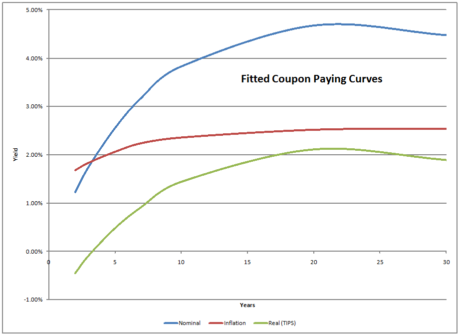
Using closing prices, here is my estimate of the coupon-paying yield curve:
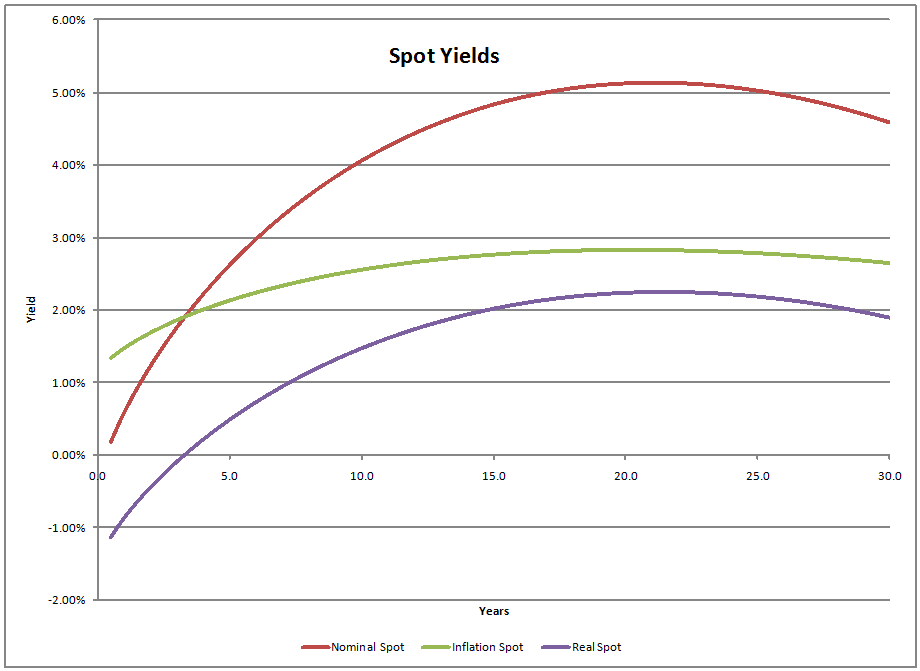
And here is the spot curve (estimating where zero coupon bonds would price):
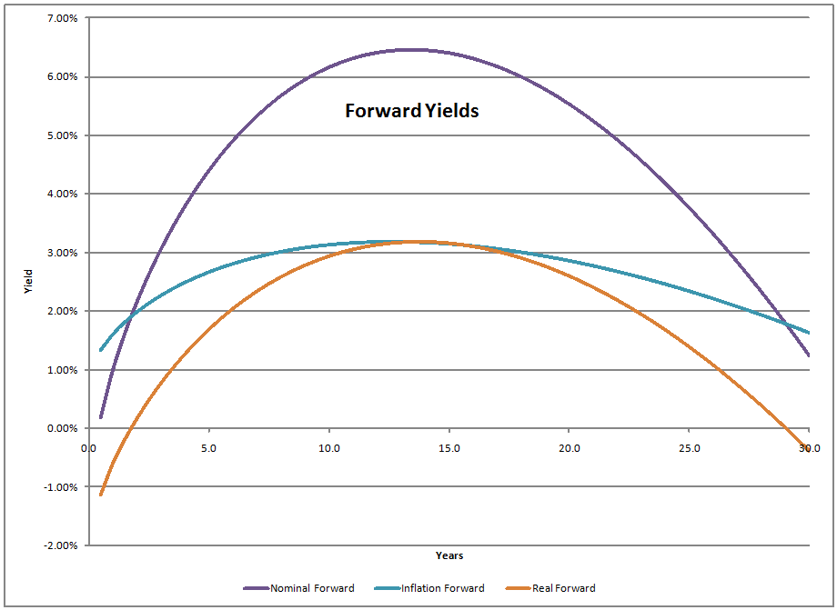
And finally, the forward curve, which estimates the expectations of future short-term rates, inflation, and real rates:
Pretty neat, huh?? Let me tell you a little about the model:
- Values are as of the close 12/22/2009, but the model can be run in real time.
- It is estimated from the full coupon-paying Treasury Note and Bond markets — over 200 bonds in the model.
- The model estimates a nominal spot curve, fitting prices with 4 parameters, over 99% R-Squared.
- The model estimates a forward inflation curve, fitting TIPS prices with 4 parameters, over 99% R-Squared.
- The two models are estimated jointly, through nonlinear optimization.
- The model has one constraint — nominal spot yields must be positive after 4 months.
- Every other curve is derived from those two curves.
What are the useful things that we learn from the model?
- There are mispricings in the Treasury and TIPS curves, but they are typically small, and would be hard to make money off of.? That’s? demonstrated by the high R-Squareds.
- The Fed has achieved its goal of making real rates negative in the short term.
- And, has made made nominal rates negative for some very short instruments inside 6 months of maturity.
- Inflation expectations start low, and peak around 2022, then tail off.
- Long term inflation expectations are still under 3.5% — ignore the portion of the inflation and real curves after 23 years, they are extrapolations.
- Implied short-term real yields go positive in 2011, peak in 2024 and tail off thereafter.
- The nominal forward curve is steep as a mountain on both sides.? Though there is a lot of fear over what will happen over the next 12-14 years, those fears have not been built into the prices of longer-dated Treasury securities.
- The nominal spot curve peaks after 22 years — in my experience, that is normal, and is a reason why longer nominal note yields decline.? US Treasury — take note.
- Inspecting the differences between coupon-paying yields on Treasuries and TIPS makes inflation expectations look more tame than they really are.? Federal Reserve — take note.
- 30-year TIPS would likely fund cheaper than 20-year TIPS — US Treasury, take note.? The scarcity value would help as well.
This is just the beginning.? I’m not planning on writing about this every day, but I should be able give you some updates every now and then.? Hopefully the firm I work for should be able to benefit through research that this enables me to create for institutional clients.
Full disclosure: I own shares in Vanguard’s TIPS fund.? And truth, we all own Treasuries somewhere if we look deep enough. 😉


David — you seem to have committed the same act as the Bear Stearns MD in your story (minus the insults). You say your model has R^2 of 99%, but you don’t say what the model is or whether your R^2 is for today’s (12/22) rates only or if it fits the data over a longer time period? You don’t say what the four mystery parameters are. You don’t give us anything other than several pretty pictures that may have come from an unknown model or may have simply been “hand drawn” in a spreadsheet.
If you are estimating a single day’s curve, R^2 99% is not impressive — the “model” is essentially just fitting a spline.
If you are estimating over a time period, I have to wonder how a single model would incorporate changing drivers. Lots of models worked in a given environment, but then failed when the economic environment shifts and the model didn’t. LTCM, Bear Stearns (and many others) learned that the hard way
At least let us see the original Bear Stearns model (assume whatever improvements you made since are proprietary — but the Bear model from 1990 is not even yours).
Greg,
It is for today’s rates only, but I have used it at other jobs — the fit is always better than 98% every day I have used it.
The paper was called “The Yield Surface,” and I probably have a paper copy lying around here somewhere, but I have no idea where. I certainly don’t have it in digital form. The formula is a modified quadratic with time as the independent variable, where the fourth coefficient multiplies onto the power of the linear and quadratic terms:
yield = a + bt^w + ct^(2w)
There. I am more generous than Mr. Diller, because figuring out what he meant from “The Yield Surface” was a chore. I didn’t publish the equations, because they are too wonky for most.
I share what I can; the rest is for my firm’s clients. But, you want the coefficients? I’ll add those — for what good it will do:
Nominal Inflation
a -0.00409 0.00914
b 0.01037 0.00782
c -0.00048 0.00067
w 0.77716 0.69568
This is not a predictive model. It is a descriptive model. But it does give some interesting conclusions, most of which I have shared.
Oh, and in principle, the US Government could use it to gauge expectations of inflation and real yields. It’s an improvement over their published models.
Very nice. Thank you. I would love to see these graphs updated periodically. Aside from that, new 30 year TIPS are coming on 2/22/2010. Jansen wrote periodically about their yield. But I have never seen a specimen so far, so I am not sure how long they have been around (if at all).
http://www.treas.gov/offices/domestic-finance/debt-management/auctions/auctions.pdf
Thank you David — I wasn’t trying to be critical. I just had trouble evaluating the model (and thus how useful it could be) without knowing anything about it. I usually don’t use any of the models from your blog (at least not as is) — but I almost always learn something from studying them.
I will have to play with the model on my own, but from the equation, it looks like a much simpler version of some cubic spline models I have seen elsewhere.
Can the model handle complex yield curves? E.G. when the yield curve is “inverted” for the first few years and then “normal” for the remaining years? The cubic spline models (which are strictly used for RV purposes, not predictive) employ several more layers to be able to handle these sorts of curves
Merry Christmas to you and your family David, and thank you for all your hard work on this blog
IF, Greg, thanks for the comments — I had forgotten about the 30-year TIPS issuance coming. I miss John Jansen too.
Yes, it can handle inverted curves. The parameters look a lot different, but it can handle those.
Though I learned how to do cubic splines when studying mortality table construction 20+ years ago, I have never used them.
One other note — these curves were used to fit bond prices, not the yield curves themselves.
Happy new year to all!
Oh, one other note — the top graph with the coupon curve — those are the yields for hypothetical par securities.
David, using the coefficients mentioned above in the nominal case, for the quadratic term, say for t=1 (year), one gets a negative number to the power 1.5ish, which doesn’t compute. Sure c is a negative number?
-0.00409 + 0.01037 * 1^0.77716 – 0.00048 * 1^(2*0.77716)
1 to any power is 1
-0.00409 + 0.01037 – 0.00048 = .00580 = 0.58%
Hi David,
I am a CFA candidate and would like to learn quantitative techniques in detail, that are used in Investment Decision Making. Could you please suggest some books that covers relevant areas??
Please Reply.
With Regards,
Hi David…very neat analysis! Do you have a book that you would recommend to buy off amazon (link off your site) that explains the forward curve/negative curves/ basically understand how bonds affect prices?
Merry X-mas
I have been searching for this paper and found a citation for
S. Diller, “The yield surface – a three dimensional approach relating yield to duration and convexity, Bear Stearns, fixed income strategies” February, New York
Is there any way we can get a copy of this paper? It doesn’t appear to be published in any journals I can find.
Secondly, how many free parameters are in the model? Are the a, b, c, w coefficients estimated from some other numerical procedure (by actually computing convexity from some other dataset)? You mentioned that you used a nonlinear fit, which is fine, but did not specify which variables are free in this fitting procedure.
Shiv and brendo — I will have a post on that soon.
David C. — I might have a copy of the paper somewhere in my basement. If I find it, I could scan it. My problem is getting the time to look for it. If you have the formula that I listed, you have the “money shot” of the paper.
There are two sets of a, b, c, and w. One for nominal Treasury rates, and the other for inflation. Eight parameters in all.
What was the data? Bond prices, coupons, and maturities and time. The idea was to estimate interest rates and implied inflation rates from the prices of Treasury securities versus their cash flows.
Here’s the equation:
This is the way I have written the from the beginning. I said a, b, c, and w before — originally they were alpha, beta, gamma and omega. It is a remarkably flexible functional form, and parsimonious. If omega is one (rare), beta and gamma become the prices for duration and convexity. Alpha is the overnight rate. Since omega is usually not one, I call beta and gamma the prices of pseudo-duration and pseudo-convexity. Under ordinary circumstances, for nominal rates, alpha, beta and omega are positive, and gamma negative.
Things are not normal for alpha now, given the government flooding the system with liquidity. Alpha would go more negative if I did not constrain spot rates after three months to be positive. I would get a better fit, but I have a hard time thinking that model is working right if I let spot rates get negative too far out.
The omega variable is what makes the functional form so flexible. It also means that the parameters can no longer be estimated through regression, but must be solved using nonlinear optimization (in Excel, using solver).
The raw data for the model is nominal Treasury note and bond, and TIPS prices. I minimize the squared error between the actual prices, and the hypothetical prices generated by discounting the cash flows of the bonds from the yields generated from the four-factor equation above. A second four-factor equation of the same form drives forward inflation estimates, and thus cash flows on the TIPS.
So, there are eight variables for this model. It’s a parsimonious system that explains a lot, and looks reasonable.
Duh, should have known that one 🙂
This form makes it much clearer. Thx. Now shouldn’t the c/gamma variable in the inflation model then be negative as well?
This is a great piece. Thanks for posting it. I would add is that theoretically, the coupon yield is related to the zero yield: e^r = zero rate
If you have a chance, I would be curious is that holds.
c/gamma was negative as I listed it for nominals above, and I commented in my last post that gamma was usually negative, yes.
Eddy, a/alpha (aleph) should be close to zero as the overnight rate in the present environment. Sadly, it is lower than that, because of the liquidity flood.