I would encourage you to have a read of the 2014 Baltimore Business Review.? Produced by the CFA Institute? — Baltimore, and Towson University, it? is a great example of how academics and practitioners can work together.? Here is my article, reformatted so that it looks better on my blog:

Differences in US States? Unemployment over the Last 36 Years

Unemployment is often treated as a national issue, but unemployment is often driven by regional or industry sector issues. This article pries apart the causes of unemployment since 1976, state-by-state.

Though there is a national component to every US state?s unemployment level, it is notable that local factors often dominate national trends. Here are some examples:

• North Dakota has an energy boom amid increasing unemployment following the housing bust in 2008.
• Texas had increasing unemployment in the mid-1980s as energy prices fell dramatically, in the midst of an economic boom.
• Coastal economies benefited during the housing boom (pre-2008), and were punished in the bust ? this is parallel to the US economy as a whole, but more severe.
• The Rust Belt prospered slowly in the early 1980s as the rest of the nation began to prosper rapidly.

The rest of this article will explain the causes of unemployment over the last 36 years, related to how connected a state is to the rest of the US economy, and how well the industry mix in a given state is doing.

Data & Method

Unemployment data for each state and the US as a whole was obtained from the St. Louis Federal Reserve?s Federal Reserve Economic Data (FRED) database. The data covers the period from 1976 to August 2013. Ordinary least squares regression was used to calculate how sensitive unemployment rates were in each state relative to overall US unemployment rates. The equation looks like this:

U_state,t = ?_state + ?_stateU_US,t + ?_state,t

The intuition behind this equation is that the unemployment rate of a given state can be explained by the amount that it varies in proportion to the unemployment rate for the US as a whole (the beta term), a fixed difference (the alpha term), and the error term. Here were the results by State:

State	Alpha	Beta	Alpha SD	Beta SD	R-squared	Alpha T-stat	Beta T-Stat	Correlation Group
Michigan	???? (2.50)	?1.67	??????? 0.25	????? 0.04	81.46%	?????????? (9.98)	???????? 17.82	3
Nevada	???? (2.44)	?1.42	??????? 0.22	????? 0.03	80.77%	???????? (11.22)	???????? 12.80	2
Indiana	???? (2.47)	?1.35	??????? 0.20	????? 0.03	81.90%	???????? (12.42)	???????? 11.63	3
Alabama	???? (1.80)	?1.32	??????? 0.23	????? 0.03	75.95%	?????????? (7.72)	????????? 9.06	6
West Virginia	????? 0.28	?1.24	??????? 0.48	????? 0.07	40.15%	??????????? 0.59*	????????? 3.42	6
Ohio	???? (1.10)	?1.23	??????? 0.17	????? 0.03	83.93%	?????????? (6.49)	????????? 9.21	3
Rhode Island	???? (1.03)	?1.17	??????? 0.26	????? 0.04	65.95%	?????????? (3.88)	????????? 4.33	5
Illinois	???? (0.51)	?1.17	??????? 0.14	????? 0.02	87.48%	?????????? (3.64)	????????? 8.08	3
Tennessee	???? (0.86)	?1.17	??????? 0.15	????? 0.02	85.25%	?????????? (5.65)	????????? 7.29	3
North Carolina	???? (1.44)	?1.14	??????? 0.19	????? 0.03	77.35%	?????????? (7.40)	????????? 4.85	2
Oregon	???? (0.00)	?1.13	??????? 0.17	????? 0.03	80.95%	?????????? (0.03)*	????????? 5.11	3
South Carolina	???? (0.72)	?1.13	??????? 0.18	????? 0.03	79.11%	?????????? (3.94)	????????? 4.69	2
California	????? 0.20	?1.12	??????? 0.18	????? 0.03	79.43%	??????????? 1.14*	????????? 4.61	5
Washington	????? 0.07	?1.09	??????? 0.15	????? 0.02	83.84%	??????????? 0.49*	????????? 3.98	6
Florida	???? (0.53)	?1.07	??????? 0.18	????? 0.03	78.09%	?????????? (2.93)	????????? 2.80	5
Pennsylvania	???? (0.33)	?1.07	??????? 0.14	????? 0.02	85.43%	?????????? (2.40)	????????? 3.52	6
Wisconsin	???? (1.30)	?1.07	??????? 0.17	????? 0.03	78.88%	?????????? (7.49)	????????? 2.57	3
Arizona	???? (0.50)	?1.06	??????? 0.18	????? 0.03	77.62%	?????????? (2.81)	????????? 2.28	2
Kentucky	????? 0.20	?1.05	??????? 0.20	????? 0.03	72.97%	??????????? 1.00*	????????? 1.56*	3
New Jersey	???? (0.10)	?1.01	??????? 0.21	????? 0.03	68.87%	?????????? (0.47)*	????????? 0.32*	5
Mississippi	????? 1.57	?0.99	??????? 0.27	????? 0.04	57.37%	??????????? 5.86	???????? (0.29)*	3
Missouri	???? (0.28)	?0.97	??????? 0.12	????? 0.02	86.47%	?????????? (2.35)	???????? (1.54)*	4
Georgia	???? (0.22)	?0.96	??????? 0.16	????? 0.02	78.07%	?????????? (1.37)*	???????? (1.81)*	2
Delaware	???? (0.83)	?0.95	??????? 0.20	????? 0.03	67.93%	?????????? (4.05)	???????? (1.73)*	1
Connecticut	???? (0.41)	?0.91	??????? 0.23	????? 0.03	61.44%	?????????? (1.80)*	???????? (2.79)	5
Utah	???? (0.60)	?0.88	??????? 0.15	????? 0.02	76.69%	?????????? (3.91)	???????? (5.13)	3
Idaho	????? 0.36	?0.88	??????? 0.20	????? 0.03	65.13%	??????????? 1.77*	???????? (4.09)	6
Colorado	???? (0.01)	?0.87	??????? 0.17	????? 0.03	71.86%	?????????? (0.04)*	???????? (5.06)	4
Maine	????? 0.31	?0.87	??????? 0.19	????? 0.03	66.45%	??????????? 1.61*	???????? (4.49)	1
Massachusetts	????? 0.17	?0.86	??????? 0.24	????? 0.04	55.28%	??????????? 0.72*	???????? (3.94)	5
Minnesota	???? (0.29)	?0.82	??????? 0.12	????? 0.02	82.17%	?????????? (2.43)	???????? (9.78)	3
District of Columbia	????? 2.45	?0.81	??????? 0.18	????? 0.03	66.11%	????????? 13.40	???????? (6.86)	1
New York	????? 1.48	?0.81	??????? 0.18	????? 0.03	67.90%	??????????? 8.45	???????? (7.28)	1
Arkansas	????? 1.46	?0.79	??????? 0.18	????? 0.03	66.27%	??????????? 8.23	???????? (7.87)	6
Virginia	???? (0.30)	?0.78	??????? 0.08	????? 0.01	90.79%	?????????? (3.84)	??????? (18.90)	1
Maryland	????? 0.31	?0.78	??????? 0.12	????? 0.02	81.92%	??????????? 2.66	??????? (12.83)	1
Iowa	???? (0.17)	?0.77	??????? 0.19	????? 0.03	61.15%	?????????? (0.86)*	???????? (7.98)	3
Vermont	????? 0.06	?0.74	??????? 0.19	????? 0.03	60.28%	??????????? 0.34*	???????? (9.04)	1
Louisiana	????? 2.45	?0.73	??????? 0.38	????? 0.06	26.41%	??????????? 6.40	???????? (4.69)	6
New Hampshire	????? 0.12	?0.68	??????? 0.20	????? 0.03	52.48%	??????????? 0.60*	??????? (10.73)	1
New Mexico	????? 2.67	?0.64	??????? 0.21	????? 0.03	48.44%	????????? 12.78	??????? (11.36)	6
Montana	????? 1.84	?0.61	??????? 0.21	????? 0.03	45.25%	??????????? 8.65	??????? (12.16)	6
Oklahoma	????? 1.49	?0.59	??????? 0.22	????? 0.03	41.23%	??????????? 6.70	??????? (12.25)	3
Wyoming	????? 1.48	?0.56	??????? 0.29	????? 0.04	26.35%	??????????? 5.08	??????? (10.17)	3
Alaska	????? 4.52	?0.53	??????? 0.28	????? 0.04	25.87%	????????? 16.05	??????? (11.13)	6
Hawaii	????? 1.46	?0.52	??????? 0.27	????? 0.04	27.58%	??????????? 5.52	??????? (12.07)	1
Texas	????? 2.89	?0.52	??????? 0.19	????? 0.03	41.71%	????????? 15.10	??????? (16.90)	4
Kansas	????? 1.68	?0.48	??????? 0.13	????? 0.02	55.86%	????????? 12.53	??????? (25.79)	4
Nebraska	????? 0.61	?0.46	??????? 0.13	????? 0.02	54.10%	??????????? 4.62	??????? (27.48)	3
South Dakota	????? 0.95	?0.45	??????? 0.11	????? 0.02	63.95%	??????????? 8.93	??????? (34.82)	3
North Dakota	????? 1.49	?0.39	??????? 0.18	????? 0.03	31.54%	??????????? 8.14	??????? (22.19)	6

* Indicates not statistically significant from zero for alpha, and one for beta at a 5% level.

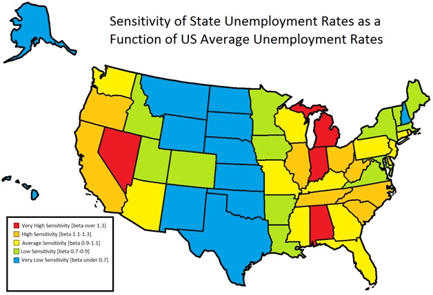
The difference in sensitivity to the US unemployment rate is considerable by state. If the unemployment rate rose 1% in the US, Michigan?s unemployment rate would tend to rise 1.67%, while the North Dakota?s unemployment rate would only tend to rise 0.39%.

The states were then divided into five beta groups, symmetric around 1.0, with a width of 0.2 for the three middle groups. On a map, it looks like this:

 

The highest sensitivity states to US unemployment rates are largely found in states with high exposure to the Auto and Gambling industries. When times are bad, people shepherd their money more carefully. They cut back on buying new cars, and gambling. High sensitivity states tend to have a lot of gearing to industrial activity, which tends to be more boom-bust than other economic activity. Average sensitivity states tend to have balanced economies, reflecting a mix of business similar to that of the US as a whole. Low-sensitivity states tend to have a large amount agriculture, resource extraction, financial sector concentration, or Federal government work.

Note that the recent boom and bust would argue that financials are more cyclical than previously believed, but that was during a small period during the study period.? The same applies in reverse to agriculture and resource extraction, which benefited from increased demand for raw materials from the developing world, making these industries appear less cyclical than previously believed.

Betas reflect the overall sensitivity to moves in US unemployment rates from 1976 to 2013, but the correlation of the residuals of the states highlight hidden factors that were influential in unemployment rate movements.

Typically, the factors stemmed from the economic sectors prominent in each group of states, as their profitability waxed and waned.

Starting with ten groups of states randomly divided, the groups were iteratively adjusted, combining groups that were highly correlated with each other until there were no more improvements possible, ending with six groups. Here is the average correlation matrix:

 

Avg Corr	1	2	3	4	5	6
Group 1	40%
Group 2	-4%	43%
Group 3	-34%	-15%	43%
Group 4	-37%	12%	24%	36%
Group 5	41%	26%	-51%	-22%	61%
Group 6	-14%	-43%	30%	-5%	-46%	50%

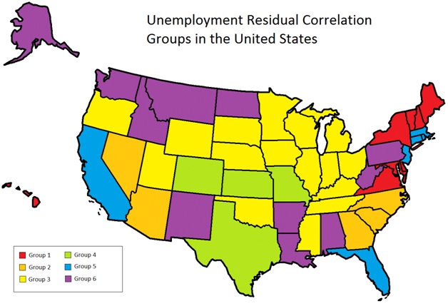
And here is the map identifying the groups:

Groups 1, 2 and 5 correlate strongly internally and moderately among each other. The same is true for 3, 4 and 6. The rest of the group correlations are weak if not negative.

Groups 3, 4, and 6 cover the center of the US. They have proportionately more economic sectors in agriculture, energy, consumer cyclicals, and basic materials.? Much of the area is rural. Groups 1, 2 and 5 cover the coasts of the US and are more heavily urbanized. Their economic sectors have a greater proportion of finance, healthcare, and technology.? Post-2007 unemployment was relatively worse in groups 1, 2 and 5 versus the other groups, because they were part of the hot housing markets, and lost more construction jobs as a result.

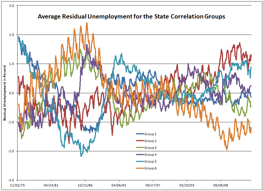
Here is a graph of the average unemployment residuals for the six correlation groups over the 36-year study period:

Description of the Correlation Groups

Group 1 ? composed of Maryland, other Mid-Atlantic States, New England and Hawaii, this ? had high unemployment relative to the rest of the US in 1976 and 1997, and low unemployment in 1987. It has high relative exposure to the consumer noncyclicals and financials sectors, and low relative exposure to energy and technology. The high weight in financials helps explain the employment gains from 1976 to 1987, as financial companies benefited from falling interest rates, rising equity markets, and expanding product offerings.

Group 2 ? composed of the Carolinas, Georgia, Arizona and Nevada ? had high unemployment relative to the rest of the US in 2011, and low unemployment in 1984 and 1991. It has a lot of relative exposure to the consumer noncyclicals and utilities sectors, and low relative exposure to energy, financials, and technology.? During the mid-1980s to early 1990s, this group benefited from the growth in demand for noncyclical goods from the Baby Boomers. After the popping of the financial bubble in 2008, weakness in construction and gambling in Arizona and Nevada led to higher levels of unemployment.

Group 3 ? composed of the Midwest, parts of the South, Utah and Oregon ? had high unemployment relative to the rest of the US in 1976 and 1992, and low unemployment in 1986. It has high relative exposure to the consumer cyclicals and noncyclicals and basic materials sectors, and low relative exposure to energy and technology. The US economy as a whole peaked and troughed along with group 3, which makes sense given their relatively large exposure to cyclical sectors.

Group 4 ? composed of Texas, Missouri, Kansas and Colorado ? had high unemployment relative to the rest of the rest of the US in 1987 and 2003, and low unemployment in 1976. It has a lot of relative exposure to the energy and utilities sectors, and low relative exposure to financials and technology. Performance of the energy sector is the critical factor here ? it was relatively strong in the mid-to late 1970s, but weak after oil prices bottomed out in the mid-1980s and late 1990s.

Group 5 ? composed of the densely populated coastal states of California, Florida, New Jersey, Massachusetts, Connecticut and Rhode Island ? had high unemployment relative to the rest of the rest of the US in 1976, 1992 and 2012, and low unemployment in 1986. It has a lot of relative exposure to the healthcare and technology sectors, and low relative exposure to energy and consumer noncyclicals. In the early 1990s, the aerospace industry in California went bust while the commercial property markets were at the deepest point of their slump. Most of the rest of the unemployment cyclicality can be attributed to the more cyclical nature of the industries in this group ? an amplified version of the US economy.

Group 6 looks like a bunch of leftovers, but it is not.? Composed of states in the Northwest and Alaska, New Mexico, Louisiana, Arkansas and Alabama, West Virginia and Pennsylvania, this group had high unemployment relative to the rest of the rest of the US in 1987, and low unemployment in 1976 and 2009.? It has a lot of relative exposure to the agriculture and basic materials sectors, and low relative exposure to financials. The stagflation of the mid-1970s benefited agriculture and basic materials, as did growth in demand from emerging markets in 2009. Those factors were
absent in 1987, as financial firms were booming.

Maryland?s unemployment rates have held down well being next to Washington, DC. The growth in the US government during the last 10 years has supported employment in Maryland. The grand question to ponder is what would ever happen to Maryland, Washington, DC and Virginia if significant cuts were made to Federal payrolls?

Conclusion

There are two main conclusions:

1) State level unemployment is a result of sensitivity to US unemployment levels and the mix of local industries. Policymakers should know how sensitive their state is to the national economy, and what industries are doing well or poorly before taking credit for low unemployment rates. More often than not, the employment rates are low or high due to factors beyond the control of policymakers.

2) In general, greater employment stability exists when that industry mix is more diversified. This is something policymakers can limitedly affect. Most states have efforts to attract businesses to their states. If you want unemployment levels to be more stable, aim your efforts at attracting businesses that diversify your existing mix.