Search Results for “dollar weighted returns”

We Eat Dollar Weighted Returns ? III (Update)

Posted on 6 November 20196 November 2019 by David Merkel

Photo Credit: Sitoo || No, you can’t eat money. But without money farmers would have a hard time buying what they need to grow crops, and we would have a hard time bartering to buy the crops

Tonight I am going to talk about one of the most underrated concepts in finance — the difference between dollar-weighted and time-weighted returns, and why it matters.

So far on this topic, I have done at least seven articles in this series, and you can find them here. The particular article that I am updating is number 3, which deals with the granddaddy of all ETFs, the SPDR S&P 500 ETF (SPY), which has been around now for almost 27 years. It is the largest ETF in the world, as far as I know.

From the end of January 1993 to the end of March 2019, SPY returned 9.42%/year on a time-weighted or total return basis. What that means is that if you had bought at the beginning and held until the end, you would have received an annualized return of 9.42%. Pretty good I say, and that is an advertisement for buy and hold investing. It is usually one of the top investing strategies, and anyone can do it if they can control their emotions.

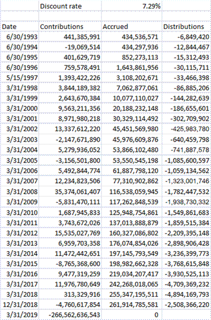
Over the same period, SPY returned 7.29%/year on a dollar-weighted basis. What this means is if you took every dollar invested in the fund and calculated what it earned over the timespan being analyzed, they would have received an annualized return of 7.29%.

That’s an annualized difference of 2.13%/year over a 26+ year period. That is a serious difference. Why? Where does the difference come from? It comes partially from greed, but mostly from panic. More shares of SPY get created near market peaks when everyone is bullish, and fewer get created, or more get liquidated near market bottoms. Many investors buy high and sell low — that is where the difference comes from. This also is an advertisement for buy and hold investing, albeit a negative one — “Don’t Let This Happen To You.”

Comparison with the 2012 Article

Now, I know few people actually look at the old articles when I link to them. But for the sharp readers who do, they might ask, “Hey, wait a minute. In the old article, the difference was much larger. Time-weighted was 7.09%/year and dollar-weighted was 0.01%/year. Why did the difference shrink?” Good question.

The differences between time- and dollar-weighted returns stems mostly from behavior at turning points. As I have pointed out in prior articles, typically the size of the difference varies with the overall volatility of the fund. People get greedy and panic more with high-volatility investments, and not with low-volatility investments.

That said, most of the effects of the difference are created at the turning points. During the midst of a big move up or down, the amount of difference between dollar- and time-weight returns is relatively small. The big differences get created near the top (buying) and the bottom (selling).

So, since the article in 2012, the fund has grown from $80 billion to over $260 billion at the end of March 2019. There have been no major pullbacks in that time — it has been a continuous bull market. We will get to see greater divergence after the next bear market starts.

Be Careful what you Read about Dollar-Weighted Returns

I’m not naming names, but there are many out there, even among academics that are doing dollar-weighted returns wrong. They think that differences as cited in my articles are too large and wrong.

The idea behind dollar-weighted return is to run an Internal Rate of Return calculation. To do that you have to have a list of the inflows and outflows by date, together with the market value of the fund at the end as an outflow, and calculate the single rate that discounts the net present value of all the flows to zero. That rate is the dollar-weighted return, and you can use the XIRR function is Excel to help you calculate it. (Note that my calculations use a mid-period assumption for when the cash flows.)

The error I have seen is that they try to make the dollar-weighted calculation like that of the time-weighted, creating period by period values. Now, there is a way to do that, and you can see that in the appendix below. As far as I can tell, they are not doing what I will write in the Appendix. Instead, they treat each year like its own separate investing period and calculate the IRR of that year only, and then daisy-chain them like annual returns for a time-weighted calculation.

Now, the time-weighted calculation does not care at all about investor-driven cash flows, like purchases and sales of fund shares, aside from dividend payments and things like that. It does not care about the size of the fund. It just wants to calculate what return a buy and hold investor gets. [Just remember the rule that an NAV must be calculated any time there is a cash flow of any sort, otherwise some inequity takes place.]

The dollar-weighted calculation cares about all investor cash flows, and ultimately about the size of the fund at the end of the calculation. It doesn’t care about when the returns are earned, but only when the cash flows in and out of the investment.

The odd hybrid method is neither fish nor fowl. Time-weighted corresponds to buy and hold, and dollar-weighted to the returns generated by each dollar in the fund. The hybrid says something like this: “We will calculate the IRR each year, but then normalize the fund size each year to the same starting level so that the fund flows at tops and bottoms do not compound. Then we show them year-by-year so that the returns are comparable to the total returns for each year.

As H. L. Mencken said:

Explanations exist; they have existed for all time;?there is always a well-known solution to every human problem?neat, plausible, and wrong.
Source: Quote Investigator citing Mencken’s book “Prejudices: Second Series”

In an effort to make a simple annual comparison between the two, they eradicate most of the effects of selling low and buying high. More in the Appendix.

Summary

Be aware of the difference between dollar-weighted and time-weighted returns. If you have a strong control on your emotions, this is not as important. If you tend to panic, this is very important. It is more important if you buy highly volatile investments, and less so if you size your volatility to your ability to bear it.

To fund managers I would say this: if you are tired of all of the inflows and outflows, and are tired of getting whipsawed by your clients, maybe you should take a step back and lower the overall risks you are taking. This will benefit both you and your clients.

Appendix

Here’s how to run an annual calculation of dollar weighted returns that be correct. For purposes of simplicity, I will assume a simple annual calculation that has multiple cash flows inside it. (If we are working with a US-based mutual fund, there would be reporting of change in net assets every six months.)

Calculate the first year (dw1) the way the hybrid method does. No difference yet. Then for the second year, run the IRR calculation for the full two-year period (IRR2). Then the second year only dollar-weighted return (dw2) would be:

((1+ IRR2) ^2) / (1+dw1) -1 = dw2

and for each successive period it would be:

(1+IRR[n])^n(1+IRR[n-1])^(n-1) – 1 = dw[n]

That is more complex than what they do, but it would preserve the truths that each entail. It would make the values for the yearly dollar-weighted returns look odd, but hey, you can’t have everything, and the truth sometimes hurts.

Full disclosure: a few of my clients are short SPY as part of a hedged strategy.

We Eat Dollar Weighted Returns ? VII

Posted on 8 December 2015 by David Merkel

I intended on writing this at some point, but Dr. Wesley Gray (an acquaintance of mine, and whom I respect) beat me to the punch. ?As he said in his blog post at The Wall Street Journal’s The Experts blog:

WESLEY GRAY: Imagine the following theoretical investment opportunity: Investors can invest in a fund that will beat the market by 5% a year over the next 10 years. Of course, there is the catch: The path to outperformance will involve a five-year stretch of poor relative performance.? ?No problem,? you might think?buy and hold and ignore the short-term noise.

Easier said than done.

Consider Ken Heebner, who ran the CGM Focus Fund, a diversified mutual fund that gained 18% annually, and was Morningstar Inc.?s highest performer of the decade ending in 2009. The CGM Focus fund, in many respects, resembled the theoretical opportunity outlined above. But the story didn?t end there: The average investor in the fund lost 11% annually over the period.

What happened? The massive divergence in the fund?s performance and what the typical fund investor actually earned can be explained by the ?behavioral return gap.?

The behavioral return gap works as follows: During periods of strong fund performance, investors pile in, but when fund performance is at its worst, short-sighted investors redeem in droves. Thus, despite a fund?s sound long-term process, the ?dollar-weighted? returns, or returns actually achieved by investors in the fund, lag substantially.

In other words, fund managers can deliver a great long-term strategy, but investors can still lose.

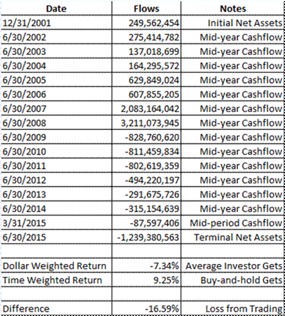
That’s why I wanted to write this post. ?Ken Heebner is a really bright guy, and has the strength of his convictions, but his investors don’t in general have similar strength of convictions. ?As such, his investors buy high and sell low with his funds. ?The graph at the left is from the CGM Focus Fund, as far back as I could get the data at the SEC’s EDGAR database. ?The fund goes all the way back to late 1997, and had a tremendous start for which I can’t find the cash flow data.

The column marked flows corresponds to a figure called “Change in net assets derived from capital share transactions” from the Statement of Changes in Net Assets in the annual and semi-annual reports. ?This is all public data, but somewhat difficult to aggregate. ?I do it by hand.

I use annual cashflows for most of the calculation. ?For the buy and hold return, i got the data from Yahoo Finance, which got it from Morningstar.

Note the pattern of cashflows is positive until?the financial crisis, and negative thereafter. ?Also note that more has gone into the fund than has come out, and thus the average investor has lost money. ?The buy-and-hold investor has made money, what precious few were able to do that, much less rebalance.

This would be an ideal fund to rebalance. ?Talented manager, will do well over time. ?Add money when he does badly, take money out when he does well. ?Would make a ton of sense. ?Why doesn’t it happen? ?Why doesn’t at least buy-and-hold happen?

It doesn’t happen because there is a Asset-Liability mismatch. ?It doesn’t matter what the retail investors say their time horizon is, the truth is it is very short. ?If you underperform for less?than a few years, they yank funds. ?The poetic justice is that they yank the funds just as the performance is about to turn.

Practically, the time horizon of an average investor in mutual funds is inversely proportional to the volatility of the funds they invest in. ?It takes a certain amount of outperformance (whether relative or absolute) to get them in, and a certain amount of underperformance to get them out. ?The more volatile the fund, the more rapidly that happens. ?And Ken Heebner is so volatile that the only thing faster than his clients coming and going, is how rapidly he turns the portfolio over, which is once every 4-5 months.

Pretty astounding I think. ?This highlights two main facts about retail investing that can’t be denied.

Asset prices move a lot more than fundamentals, and
Most investors chase performance

These two factors lie behind most of the losses that retail investors suffer over the long run, not active management fees. ?remember as well that passive investing does not protect retail investors from themselves. ?I have done the same analyses with passive portfolios — the results are the same, proportionate to volatility.

I know buy-and-hold gets a bad rap, and it is not deserved. ?Take a few of my pieces from the past:

If you are a retail investor, the best thing you can do is set an asset allocation between risky and safe assets. ?If you want a spit-in-the-wind estimate use 120 minus your age for the percentage in risky assets, and the rest in safe assets. ?Rebalance to those percentages yearly. ?If you do that, you will not get caught in the cycle of greed and panic, and you will benefit from the madness of strangers who get greedy and panic with abandon. ?(Why 120? ?End of the mortality table. 😉 Take it from an investment actuary. 😉 We’re the best-kept secret in the financial markets. 😀 )

Okay, gotta close this off. ?This is not the last of this series. ?I will do more dollar-weighted returns. ?As far as retail investing goes, it is the most important issue. ?Period.

We Eat Dollar Weighted Returns ? VI

Posted on 22 July 201522 July 2015 by David Merkel

One of the constants in investing is that average investors show up late to the party or to the crisis. ?Unlike many gatherings where it may be cool to be fashionably late, in investing it tends to mean you earn less and lose more, which is definitely not cool.

One reason why this happens is that information gets distributed in lumps. ?We don’t notice things in real time, partly because we’re not paying attention to the small changes that are happening. ?But after enough time passes, a few people notice a trend. ?After a while longer, still more people notice the trend, and it might get mentioned in some special purpose publications, blogs, etc. ?More time elapses and it becomes a topic of conversation, and articles make it into the broad financial press. ?The final phase is when?general interest magazines put it onto the cover, and get rich quick articles and books point at how great fortunes have been made, and you can do it too!

That slow dissemination and?gathering of information is paralleled by a similar flow of money, and just as the audience gets wider, the flow of money gets bigger. ?As the flow of money in or out gets bigger, prices tend to overshoot fair value, leaving those who arrived last with subpar returns.

There is another aspect to this, and that stems from the way that people commonly evaluate managers. ?We use past returns as a prologue to what is assumed to be still?greater returns in the future. ?This not only applies to retail investors but also many institutional investors. ?Somme institutional investors will balk at this conclusion, but my experience in talking with institutional investors has been that though they look at many of the right forward looking indicators of manager quality, almost none of them will hire a manager that has the right people, process, etc., and has below average returns relative to peers or indexes. ?(This also happens with hedge funds… there is nothing special in fund analysis there.)

For the retail crowd it is worse, because?most investors look at past returns when evaluating managers. ?Much as Morningstar is trying to do the right thing, and have forward looking analyst ratings (gold, silver, bronze, neutral and negative), yet much of the investing public will not touch a fund unless it has four or five stars from Morningstar, which is a backward looking rating. ?This not only applies to individuals, but also committees that choose funds for defined contribution plans. ?If they don’t choose the funds with four or five stars, they get complaints, or participants don’t use the funds.

Another Exercise in Dollar-Weighted Returns

One of the ways this investing shortfall gets expressed is looking at the difference between time-weighted (buy-and-hold) and dollar-weighted (weighted geometric average/IRR) returns. ?The first reveals what an investor who bought and held from the beginning earned, versus what the average dollar invested earned. ?Since money tends to come after good returns have been achieved, and money tends to leave after bad returns have been realized, the time-weighted returns are typically higher then the dollar-weighted returns. ?Generally, the more volatile the performance of the investment vehicle the larger the difference between time- and dollar-weighted returns gets. ?The greed and fear cycle is bigger when there is more volatility, and people buy and sell at the wrong times to a greater degree.

(An aside: much as some pooh-pooh buy-and-hold investing, it generally beats those who trade. ?There may be intelligent ways to trade, but they are always a minority among market actors.)

HSGFX Dollar Weighted Returns — HSGFX Dollar and Time Weighted Returns

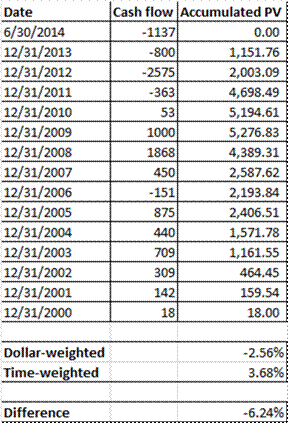
That brings me to tonight’s fund for analysis: Hussman Strategic Growth [HSGFX]. John Hussman, a very bright guy, has been trying to do something very difficult — time the markets. ?The results started out promising, attracting assets in the process, and then didn’t do so well, and assets have slowly left. ?For my calculation this evening, I run the calculation on his fund with the longest track record from inception to 30 June 2014. ?The fund’s fiscal years end on June 30th, and so I assume cash flows occur at mid-year as a simplifying assumption. ?At the end of the scenario, 30 June 2014, I assume that all of the funds remaining get paid out.

To run this calculation, I do what I have always done, gone to the SEC EDGAR website and look at the annual reports, particularly the section called “Statements of Changes in Net Assets.” ?The cash flow for each fiscal year is equal to the?net increase in net assets from capital share transactions plus the net decrease in net assets from distributions to shareholders. ?Once I have?the amount of money moving in or out of the fund in each fiscal year, I can then run an internal rate of return calculation to get the dollar-weighted rate of return.

In my table, the cash flows into/(out of) the fund are in millions of dollars, and the column titled Accumulated PV is the?accumulated present value calculated at an annualized rate of -2.56% per year, which is the dollar-weighted rate of return. ?The zero figure at the top shows that a discount rate -2.56% makes the cash inflows and outflows net to zero.

From the beginning of the Annual Report for the fiscal year ended in June 2014, they helpfully provide the buy-and-hold return since inception, which was +3.68%. ?That gives a difference of 6.24% of how much average investors earned less than the buy-and-hold investors. ?This is not meant to be a criticism of Hussman’s performance or methods, but simply a demonstration that a lot of people invested money after the fund’s good years, and then removed money after years of underperformance. ?They timed their investment in a market-timing fund poorly.

Now, Hussman’s fund may do better when the boom/bust cycle turns if his system makes the right move?somewhere near the bottom of the cycle. ?That didn’t happen in 2009, and thus the present state of affairs. ?I am reluctant to criticize, though, because I tried running a strategy like this for some of my own clients and did not do well at it. ?But when I realized that I did not have the personal ability/willingness to?buy when valuations were high even though the model said to do so because of momentum, rather than compound an error, I shut down the product, and refunded some fees.

One thing I can say with reasonable confidence, though: the low returns of the past by themselves are not a reason to not invest in Mr. Hussman’s funds. ?Past returns by themselves tell you almost nothing about future returns. ?The hard questions with a fund like this are: when will the cycle turn from bullish to bearish? ?(So that you can decide how long you are willing to sit on the sidelines), and when the cycle turns from bearish to bullish, will Mr. Hussman make the right decision then?

Those questions are impossible to answer with any precision, but at least those are the right questions to ask. ?What, you’d rather have the answer to a simple question like how did it return?in the past, that has no bearing on how the fund will do in the future? ?Sadly, that is the answer that propels more investment decisions than any other, and it is what leads to bad overall investment returns on average.

PS — In future articles in this irregular series, I will apply this to the Financial Sector Spider [XLF], and perhaps some fund of Kenneth Heebner’s. ?Till then.

We Eat Dollar Weighted Returns ? V

Posted on 18 September 2012 by David Merkel

This is the first episode of “We Eat Dollar Weighted Returns” where the fare is yummy.? Here’s the twist: investors in some bond ETFs have done better than one who bought at the beginning and held.

Now, all of this is history-dependent.? The particular bond funds I chose were among the largest and most well-known bond ETFs — HYG (iShares iBoxx $ High Yield Corporate Bd), JNK (SPDR Barclays Capital High Yield Bond), and TLT (iShares Barclays 20+ Year Treas Bond).

As bond funds go, these are relatively volatile.? TLT buys the longest Treasury bonds, taking interest rate risk.? HYG and JNK buy junk bonds, taking credit risk.

Let’s start with TLT:

Date	Cash Flow	Buy & Hold Return	Cumulated
11/9/2002	248,935,892		1
8/31/2003	-73,889,166	12.31%	1.1231
8/31/2004	439,348,999	3.11%	1.15802841
8/31/2005	73,509,821	6.72%	1.235847919
8/31/2006	442,211,811	6.12%	1.311481812
8/31/2007	165,784,828	3.37%	1.355678749
8/31/2008	-344,202,681	9.54%	1.485010502
8/31/2009	887,336,789	12.30%	1.667666793
8/31/2010	120,142,522	-5.85%	1.570108286
8/31/2011	-452,062,384	4.64%	1.64296131
2/29/2012	-3,038,265,474	32.32%	2.173966406

	IRR	Buy & Hold	Difference
	11.47%	8.42%	3.05%

I analyzed this back in June, saw the anomalous result, an decide to sit on it until I had more time to analyze it.? The way to think about it is that investors reached for yield at a time when stocks were in trouble, and indeed, rates went lower.? The average investor beat buy-and-hold by 3%.

Here are the results for the junk ETFs:

HYG	4/4/2007	2/29/2008	2/28/2009	2/28/2010	2/28/2011	2/29/2012

Distributions		-9,708	-92,708	-358,324	-512,979	-694,209
Net Additions		371,140	1,989,303	1,781,425	3,201,608	5,840,594
Net Assets		352,636	2,089,054	4,611,414	8,257,928	14,258,718
Investment Return		-8,796	-160,176	1,099,260	957,884	854,406
ROA		-4.57%	-13.12%	32.81%	14.89%	7.59%

	4/4/2007	9/16/2007	8/29/2008	8/29/2009	8/29/2010	8/30/2011	2/29/2012
13.40%	IRR	-361,432	-1,896,594	-1,423,100	-2,688,629	-5,146,384	14,258,718
6.04%	Buy-and hold
7.36%	Difference

JNK	11/28/2007	6/30/2008	6/30/2009	6/30/2010	6/30/2011	6/30/2012

Distributions		-9,011	-111,409	-361,521	-616,525	-735,822
Net Additions		404,658	1,481,309	2,180,582	2,366,102	3,928,526
Net Assets		394,346	1,900,709	4,301,252	6,915,538	10,780,535
Investment Return		-1,302	136,463	581,481	864,710	672,292
ROA		-0.61%	11.89%	18.75%	15.42%	7.60%

IRR	11/28/2007	3/14/2008	12/29/2008	12/29/2009	12/29/2010	12/30/2011	6/30/2012
13.22%	IRR	-395,648	-1,369,900	-1,819,061	-1,749,577	-3,192,704	10,780,535
6.49%	Buy-and hold
6.73%	Difference

Both funds were small in advance of the credit crisis, and investors bought into them as yields spiked, and bought even more as income opportunities diminished largely due to the Fed’s low-rate monetary policies. The average investor beat buy-and-hold by 6%+.

Now, the? junk funds were small during default, and grew during the boom, amid unprecedented monetary [policy from the Fed.? (Note: I think that Bernanke will rank below Greenspan in the history books in 210o, and both will be judged to be horrendous failures.? It is better to let things fail, and clear out the bad debt, rather than continue malinvestment.? We need fewer banks, houses, and auto companies, among others.? The government, including the Fed and the GSEs, should not be in the lending business.? Lending should be unusual, and applied mostly to financing short-term assets.? Long-term assets should be financed by equity, or at worst, long-dated debt.

For all three funds, we have the historical accident that the Fed dropped Fed funds rates to near zero, leading to a yield frenzy.? But what happens when defaults spike?? What? happens when no one want to buy long dated Treasuries at anything near current levels?

I think bond investors are more rational than stock investors; they have more rational benchmarks to guide them.? Bond investors have cash flows to analyze against EBITDA (earnings before interest, taxes, depreciation and amortization.? Stock investors wonder at earnings, which are easily gamed.

The real question will come when we have the next credit crisis?? How many holders of HYG or JNK will run then?? Or when inflation starts to run, and the Fed stops buying long Treasury bonds, and even starts to sell them, what will happen to dollar-weighted returns then?

This is an interesting piece for bond assets in a bull market.? We need to see bear market results to truly understand what is going on.

Full disclosure: long TLT for myself and clients

We Eat Dollar Weighted Returns ? IV

Posted on 5 May 20125 May 2012 by David Merkel

I think one of the largest areas for practical investigation in finance is reviewing dollar-weighted versus time weighted returns, especially for vehicles that are traded heavily.? I am going to try to analyze one major ETF per month to see what the level of slippage is due to trading.

But if my hypothesis is wrong, I’ll post on it anyway.? The last post I did on this was on SPY, the S&P 500 Spider.? The slippage was 7%+/year.

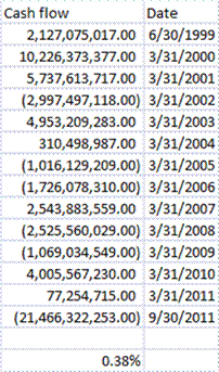
Now I have done the calculation for the QQQ, the PowerShares QQQ Trust, which mimics the Nasdaq 100.? The Nasdaq 100 is more volatile than the S&P 500, so I expected the gap to be worse, but it wasn’t: from the inception in March 1999 to the end of the fiscal year in September of 2011, the dollar weighted return was 0.38%/year versus a time-weighted return that a buy-and-hold investor would get of 0.77%/year.? 0.4% of difference isn’t much to talk about.? It still indicates a little bad trading.

That said, the net amount of unit creation and liquidation tended to be small.? Maybe that is the difference.? I have to think more about this, but my advice to anyone using exchange traded products remains the same — read your prospectus carefully, and understand the weaknesses of the vehicle.? If creation units don’t have to be something exact, ask what that might imply for your returns.

Anyway, here were the figures from my dollar-weighted return calculation:

I used annual data, and assumed midperiod dates for the cashflows.

The next ETF I plan to analyze is XLF, the Financial Sector Spider.? I suspect that will look bad, but who knows?
Full disclosure: short SPY in some hedged accounts.

We Eat Dollar Weighted Returns — III

Posted on 2 February 2012 by David Merkel

Somebody notify the Bogleheads, they will like this one, or at least Jack will.? Yo, Jack, I met you over 15 years ago at a Philadelphia Financial Analysts Society meeting.

How bad are individual investors? at investing?? Bad, very bad.? But what if we limit it to a passive vehicle like the Grandaddy of all ETFs, the S&P 500 Spider [SPY]?? Should be better, right?

I remember a study done by Morningstar, where the difference between Time and Dollar-weighted returns was 3%/year on the S&P 500 open end fund for Vanguard, 1996-2006.

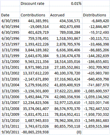
But here’s the result for the S&P 500 Spider, January 1993- September 2011.? Time-weighted return: 7.09%/year.? Dollar-weighted: 0.01%/yr.? Gap: 7%/yr+

Why so much worse than the open-end fund?? Easy.? Unlike the professional managers at Vanguard, and the relatively long term investors they attract, the retail short term traders of SPY trade badly; they arrive late, and leave late on average.

There is far more analysis to be done here, but to me, this confirms that Jack Bogle was right, and ETFs would be a net harm to retail investors.? The freedom to trade harms average investors, and maybe a lot of professionals as well.? It may also indicate that short-term trading as practiced by technicians may underperform in aggregate.? Not sure about that, but the conclusion is tempting.

One thing I will say: I am certain that profitable trading is not easy.? If you are tempted to trade for a living, the answer is probably don’t.

Anyway, here’s my spreadsheet on the topic:

Full disclosure: I have a few clients short SPY, hedged against my long positions.

We Eat Dollar-Weighted Returns

Posted on 9 October 2011 by David Merkel

Why do we do time-weighted returns for analysis of portfolios?? Because we are lazy, and they are simple to calculate.? We don’t want to be bothered with the effects of cash flows.

Besides, mutual fund managers don’t make decisions to move money in and out of their funds.? They should not be held accountable for the actions of their shareholders.

Really?? I think that is only half correct.? The good fund manager takes account of his implicit liability structure.? When will people leave, when will they come?? For almost all funds, investors are trend followers.? And the the greater the degree of volatility, the worse the investors are at following the trend.? Thus a manager of a volatile fund should run with more of a cash buffer, particularly when markets are moving down hard, because he will have more of his clients cashing out.? The manager of a volatile fund should also avoid taking concentrated positions, because when he is doing well, his own buying may drive the stocks he owns up, only to see them fall harder when he is forced to liquidate positions when the market is doing poorly, and shareholders are leaving.? Wise managers concentrate near bottoms, and diversify near tops.

Now for my poster child, the Legg Mason Value Trust.? Bill Miller is a very intelligent guy, and has a very talented staff.? My main criticism of his management is that it neglects the core concept of value investing, which is “margin of safety.”? The core concept is not cheapness, or as Bill Miller was fond of saying “lowest average cost wins.”

Legg Mason Value Trust enthused investors as they racked up significant returns in the late 90s, and the adulation persisted through 2006.? As Legg Mason Value Trust grew larger it concentrated its positions.? It also did not care much about margin of safety in financial companies.? It bought cheap, and suffered as earnings quality proved to be poor.

Eventually, holding a large portfolio of concentrated, lower-quality companies as the crisis hit, the performance fell apart, and many shareholders of the fund liquidated, exacerbating the losses of the fund, and their selling pushed the prices of their stocks down, leading to more shareholder selling.? I’m not sure the situation has stabilized, but it is probably close to doing being there.

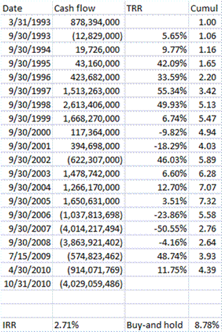
But now to the point: what did Bill Miller earn for shareholders?? The earliest date that I could get data for was 3/31/1993, probably due to the creation of EDGAR in the mid-90s.

On a dollar-weighted basis, he earned 2.71%/year for investors through 10/31/2010.? But for those stout-hearted souls that bought and held, they earned 6%+ more, 8.78%.? But those that did that had to be patient, even Stoic, people who had no need for liquidity, and no propensity for panic.? (There is always enough time to panic. 😉 )

Legg Mason Value Trust was a volatile fund, and as such, it is no surprise that the difference between time-weighted and dollar-weighted returns are so large.? But what does this imply about Bill Miller? He beat the S&P 15 years in a row.? But as posts like this point out, did he go from first to worst?

His neglect of the core idea in value investing, margin of safety, allowed him to do well as the lending bubble expanded, and low quality companies prospered.? But when the tide went out, he was found to be swimming naked.? Far from following Buffett’s principles, or Graham’s, he was just a growth investor masquerading as value investor because “he bought them cheap.”? And they got a lot cheaper, and he had to sell them cheaper still.

So what are the lessons here?

Focus on margin of safety in investing.? Analyze balance sheets.
Avoid investing in popular funds, even excellent managers make mistakes when lots of money is coming in.
Stick to your knitting.? Don’t engage in all manner of fancy logic once you achieve success.? Stay humble.
Remember that your timing in investing makes a difference.? Don’t be quick to add to a winning fund.? Better to find a fund with good ideas that is temporarily underperforming.
Buy-and-hold often beats the average investor over the long haul.? Some traders might do better, but have you developed that skill?
Avoid managers that say a lot of clever things, but can’t deliver on returns.

So be wise, and realize, you are still responsible for your investment success or failure, even if you hand it off to others.

Returns on Equity Amid the Financial Crisis

Posted on 20 December 2011 by David Merkel

I wrote the following for the 2012 Baltimore Business Review.? When it is publicly available on the web, I will highlight it.? For now, I will offer you the unedited version of my paper that will be published there:

-==-=-=-=-=-=-=-=–==-=–=-=-=-==–==-=–=-=-==-=-=-=-=-=-=-=-=-=-=-=-=-

Returns on Equity amid the Financial Crisis

Abstract

From 2005-2010, the change in public company returns on book equity [ROE] was wrenching during the financial crisis.? The results were uneven by sectors, and even by geography, for stocks traded in US equity markets.? This paper looks at the differences, and attempts to explain why there was so much variation by sector and geography.? After that, the paper attempts to explain the correlation between changes in ROE and stock returns, by year, sector, and geography.

Introduction

Since 2005, equity markets have seen a boom, a bust, and a tepid recovery. Financial stocks seem to have had the worst of it, but is that really true?

This paper attempts to disaggregate the differing effects of geography (countries/US states), and economic sector over time to try to understand how the boom, bust and recovery have affected public companies.

Part 1 ? Return on Equity

Method

This study excluded stocks with market capitalizations under $100 million at the end of the study period.? It also excluded miscellaneous financial companies such as exchange-traded products, closed-end funds, and special-purpose acquisition companies, because they don?t have operating businesses.? That left 3,796 companies that trade on US exchanges available for the analysis.

Given the tendency for businesses in states and countries to be concentrated in one or two sectors, a minimum was imposed for states and countries to be analyzed individually.? Countries with fewer than four companies trading on US exchanges were placed in the ?other? country category, and states with fewer than four companies trading on US exchanges were placed in the ?other? state category.

Over the years 2005-2010, data regarding book equity, net income, market capitalization, market price, share count, and total returns were gathered, and aggregated by geography (Country if non-US, state if US), sector, and year.

Using Ordinary Least Squares Regression, the following relationship was estimated:

Where:

?is the set of dummy variables for geography.
?is the set of dummy variables for sectors.
?is the set of dummy variables for the years 2005-2010.
?is the contribution to return on equity due to geography.
?is the contribution to return on equity due to sector.
?is the contribution to return on equity due to year.
?is the net income for a given geographic area, sector, and year.
?is the book equity for a given geographic area, sector, at the prior year end.
?is the error term for a given geographic area, sector, and year.

The reasons for using this sort of equation is twofold: first, by using dollar figures rather than earnings per share and book value per share, large companies are given their proper weight versus smaller companies.? Second, it allows for the effects of ROE changes by geography, sector and year to be separated.

In an analysis where there are multiple groups of dummy variables, at most one set of dummy variables can be complete if there is no intercept term, and no set can be complete if there is an intercept term.? If not, the regression will fail.? The choice of what to omit is arbitrary, and does not affect the relative relationships within a set of dummy variables.? For the purposes of this paper the sector dummy variables were left complete, and the coefficients on the first geographic area (Argentina) and the first year (2005) were set to zero.

Results

The R-squared of the regression was 55.7%, which has a prob-value of greater than 99.9%.

Here are the results of contribution to ROE by country:

18.1%	Mexico
16.9%	Chile
15.4%	Other Nations
15.1%	Brazil
14.1%	Australia
13.4%	Spain
13.2%	India
10.6%	Bermuda
10.6%	Hong Kong
7.3%	Greece
7.1%	Russia
6.5%	Taiwan
6.3%	Netherlands
6.3%	Italy
6.3%	Switzerland
6.1%	China
5.9%	Norway
5.8%	Canada
5.1%	Sweden
5.1%	Germany
4.1%	France
3.7%	United Kingdom
2.8%	United States
1.9%	Singapore
1.9%	Israel
1.0%	Cayman Islands
0.6%	Japan
0.1%	South Korea
0.0%	Argentina
-0.2%	Puerto Rico
-1.4%	Finland
-3.1%	Ireland
-3.2%	Luxembourg
-6.3%	South Africa

The United States is included for comparison purposes as the weighted average of the contribution to ROE by states.? There was not a separate variable for the US in the analysis.

As Latin America moved toward freer markets, with growing middle classes, their contributions to ROE were relatively high.? In general, resource rich nations tended to have higher contributions to ROE.

Mexico?s contribution to ROE was led by communication companies Telmex, America Movil, and Grupo Televisa and consumer-oriented companies like Coca-cola Femsa, FEMSA, and Wal-Mart de Mexico.? A growing middle class pushed up demand for these companies.

Chile?s contribution to ROE was led by the utilities Enersis and Empresa Nacional de Electricidad, the banks Banco Santander Chile and Banco de Chile, and chemical company Sociedad Quimica y Minera de Chile.? A growing economy boosted demand for electrical power, their banks didn?t make the mistakes made by most of the rest of the developed world, and Sociedad Quimica y Minera was in the ?sweet spot? for the chemicals it produced, particularly fertilizers, and lithium which goes into rechargeable batteries.

Brazil?s contribution to ROE was led by the energy giant Petrobras, the diversified mining company Vale, and the banks Banco Santander (Brasil), Itau Unibanco Holding, and Banco Bradesco.? Global demand for crude oil, iron ore, and other resources boosted the contributions to ROE with Petrobras and Vale.? Brazil?s banks also didn?t make the mistakes made by most of the rest of the developed world.

On the negative side, contributions to ROE in Finland were held down by Nokia, where they fell behind consumer trends with cell phones and other portable wireless devices.? Ireland was held back by banking sector, which lent too much on Irish residential property, amid other errors.? Luxembourg had ArcelorMittal, which slumped with the global steel industry as prices for coking coal and iron ore rose.? South Africa had the worst contribution to ROE as a country because of the heavy weight their economy has in basic materials.? Basic materials was a strong sector, but South Africa was concentrated in one the weakest ROE industries in that sector, gold mining.

Here are the results of contribution to ROE by US state:

18.6%	Washington
16.9%	Arkansas
13.0%	District of Columbia
11.3%	Minnesota
10.0%	Connecticut
10.0%	Oregon
8.9%	Rhode Island
8.2%	New Jersey
7.8%	Kentucky
6.7%	Nebraska
6.6%	Indiana
6.2%	California
6.1%	Georgia
5.5%	Wisconsin
5.4%	Missouri
5.1%	Iowa
5.0%	Texas
4.4%	Tennessee
3.2%	Illinois
3.1%	Florida
2.9%	Maryland
2.8%	US Average
2.5%	North Carolina
1.2%	New York
1.2%	Pennsylvania
1.1%	South Carolina
0.8%	Other
0.6%	Ohio
-0.4%	Utah
-0.5%	Nevada
-1.3%	Louisiana
-2.3%	Arizona
-3.6%	Colorado
-4.6%	Massachusetts
-5.6%	Alabama
-7.9%	Oklahoma
-10.3%	Virginia
-31.9%	Kansas
-83.6%	Michigan

To some degree, historical accidents help explain why some states have high contributions to returns on equity, and others low contributions.? Washington State has Microsoft, Amazon, and Costco, all of which started out there.? Michigan has General Motors, Ford, and Chrysler; the automobile industry has long been a big part of the state economy.

The contribution to ROE of Arkansas can be entirely attributed to Wal-Mart.? Washington, DC can largely be attributed to Danaher, though Fannie Mae pulled the contribution to ROE down considerably as it failed in 2008.

The results of Kansas are dominated by Sprint Nextel, which has been a weak competitor in wireless telephony, though YRC Worldwide also had some impact on the low contribution to ROE as it was too acquisitive heading into a major recession.? Virginia has many strong companies, but Freddie Mac pulled the contribution to ROE down with it failure in 2008.

Companies don?t move often, so attributing the differing contributions to ROE to state policies is unlikely.? In the extreme cases listed above, all of the companies listed had been headquartered in their respective states for a long time, and most had been started there.

Here are the results of contribution to ROE by sector:

25.91%	Consumer Non-Cyclical
23.31%	Basic Materials
20.20%	Energy
18.10%	Health Care
14.59%	Utilities
14.24%	Capital Goods
14.07%	Technology
10.56%	Services
10.20%	Consumer Cyclical
9.52%	Financial
4.72%	Transportation
-5.58%	Conglomerates

The end of the first decade of the new millennium was characterized by strong development around the world, with many nations clamoring for resources and non-cyclical consumer goods, which why the contribution to ROE by sector was led by Consumer Non-Cyclicals, Basic Materials, and Energy.

Conglomerates are the smallest sector, at 0.3% of total book equity, so it is difficult to draw conclusions about why it had the lowest contribution to ROE.? That said, it is difficult to manage disparate enterprises for organic operating returns.? Increases in energy costs hurt transportation ROEs, which unlike utilities, have a harder time passing the price increases through.

Financial stocks saw their contribution to ROE drop because of the financial crisis.? The contribution to ROE includes two great years 2005-2006, two horrible years 2007-2008, and two years of recovery.? The contributions to ROE in the financial sector in 2007-2008 more than erased the gains made earlier in the decade.

Contribution to ROE for Consumer Cyclicals were damaged by bad results in the Automobile industry and slumping demand as the economy went into a recession in 2008, and had a rather weak recovery in 2009-2010.

Here are the results of contribution to ROE by year:

0.00%	2005
2.04%	2006
-1.28%	2007
-18.37%	2008
-8.06%	2009
-3.72%	2010

Contribution to return on equity rose 2% over 2005 levels in 2006.? In 2007, as the stock market reached new highs and began to fall in the fourth quarter of 2007, partially because the contribution to ROE fell below 2005 and 2006 levels.

In 2008, as the financial crisis arrived, the contribution to ROE plummeted.? Much of the effect was concentrated in financial stocks, but the contribution to ROE for the market as a whole fell 17%.? In 2009 and 2010, as the recovery from the crisis progressed contribution to ROE rose each year, but still remained below the contribution to ROE that existed during the boom years 2005-2007.

Part 2 ? Total Returns

Method

The same stocks as in the first section, and the same methods were used to estimate the following relationship, using Ordinary Least Squares:

Where:

?is the set of dummy variables for geography.
?is the set of dummy variables for sectors.
?is the set of dummy variables for the years 2005-2010.
?is the contribution to total return due to geography.
?is the contribution to total return due to sector.
?is the contribution to total return due to year.
?is the dollar value of gains or losses for a given geographic area, sector, and year.
?is the market capitalization for a given geographic area, sector, at the prior year end.
?is the error term for a given geographic area, sector, and year.

The dollar value of gains or losses is calculated by the change in market capitalization, plus dividends, less the proceeds of shares issued, plus the cost of shares bought back.

Results

The R-squared of the regression was 76.7%, which has a prob-value of greater than 99.9%.

Here are the results of contribution to total return by country:

216.77%	Israel
24.53%	Chile
17.34%	Singapore
12.44%	Other Nations
11.99%	China
11.34%	Australia
10.37%	Hong Kong
8.32%	Mexico
7.62%	Bermuda
7.15%	Brazil
4.14%	Netherlands
3.41%	Germany
3.24%	Greece
2.32%	Spain
1.93%	Norway
1.72%	Italy
1.62%	United Kingdom
1.61%	Cayman Islands
1.30%	US Average
1.24%	Taiwan
1.08%	India
0.86%	France
0.76%	Switzerland
0.74%	Puerto Rico
0.13%	Finland
0.00%	Argentina
-1.44%	Russia
-3.46%	South Korea
-4.16%	Canada
-4.32%	Japan
-4.44%	Ireland
-6.19%	South Africa
-8.72%	Sweden
-17.49%	Luxembourg

The United States is included for comparison purposes as the weighted average of the contribution to ROE by states.? There was not a separate variable for the US in the analysis.

Looking at the countries at the top and the bottom, Israel benefitted from Teva Pharmaceutical, Check Point Software Technologies, and a scad of little technology companies that soared in value.? Singapore was led by Avago Technologies which has been seeing strong growth in demand for their analog semiconductor devices.

Chile, as mentioned above, contribution to total return was led by the utilities Enersis and Empresa Nacional de Electricidad, the banks Banco Santander Chile and Banco de Chile, and chemical company Sociedad Quimica y Minera de Chile.? In addition, Lan Airlines grew their net income by 150% over the whole of the study period, as a growing middle class flew more often.

Ireland, Luxembourg and South Africa were low on the contribution to ROE by countries.? Ireland?s contribution to total returns was held back by its banking sector, as mentioned previously.? The same applies to Luxembourg with ArcelorMittal.? And again, South Africa had a low contribution to total returns as a country because of the heavy weight their economy has in basic materials.? Basic materials was a strong sector, but South Africa was concentrated in one the weakest industries for total returns in that sector, gold mining.

Sweden had three large companies Ericcson (Telecommunications Equipment), Volvo (Automobiles) and Swedbank (Banking) that underperformed.? Volvo and Swedbank were in weak industries given the financial crisis, while Ericcson underperformed versus competitors in its industry.

Note that the order of the lists of contribution to ROE and contribution to total return across are similar.? The correlation of the two sets of coefficients is 1.8% — statistically indistinguishable from zero, but the rank correlation of the two sets is 62.7%, which is significantly greater than zero with 95% certainty.? The high coefficient on Israel?s contribution to total returns throws the ordinary correlation coefficient off; without Israel, the correlation would be 64.5%.

Thus it seems that contribution to ROE and contribution to total return are related across countries.

Here are the results of contribution to total return by US state:

19.12%	Oregon
15.18%	Kentucky
13.85%	Iowa
13.28%	Michigan
12.77%	Nebraska
12.53%	Arizona
11.52%	Rhode Island
9.35%	Colorado
9.24%	Texas
8.10%	Alabama
7.18%	Louisiana
7.02%	Oklahoma
6.26%	Illinois
5.58%	California
5.01%	New Jersey
4.58%	Massachusetts
3.49%	Missouri
2.62%	Maryland
2.21%	South Carolina
2.17%	Minnesota
1.56%	Utah
1.40%	Washington
1.30%	US Average
-0.02%	Wisconsin
-0.49%	Connecticut
-1.11%	New York
-1.39%	Arkansas
-2.02%	Indiana
-3.13%	Pennsylvania
-4.49%	Florida
-5.21%	Ohio
-7.04%	Tennessee
-7.76%	North Carolina
-8.19%	Kansas
-8.42%	Nevada
-12.06%	Georgia
-19.45%	Other
-21.02%	Virginia
-33.73%	District of Columbia

Oregon?s contribution to total return was high because of Nike and Precision Castparts.? Both have been based in Oregon since their founding.? The same can be said of Yum! Brands, Humana, and Brown Forman in Kentucky.? Yum Brands began with Pepsi?s purchase of Kentucky Fried Chicken, which was founded by Colonel Sanders out of home in Corbin, Kentucky in 1930.? Brown Forman was started in Kentucky in 1870 by George Garvin Brown.

Terra Nitrogen, LP was an Iowa firm from its founding until its parent company was acquired by CF industries in mid-2010.? It is counted as an Iowa firm for this study, but is now based in Illinois.

DC and Virginia have the lowest contributions to total returns because of Fannie Mae and Freddie Mac, respectively.? Georgia had a low contribution to total returns, largely due to SunTrust Banks, which holds the dubious distinction of receiving four installments of bailout cash.? Nevada had a low contribution to total returns because of their high exposure to the casino/gaming industry, which did poorly during and after the financial crisis.

All of these companies are historical accidents.? They were based in their states since their founding.

The state lists on contribution to ROE and contribution to total return across are not similar.? The correlation of the two sets of coefficients is -10.68% — statistically indistinguishable from zero.? The rank correlation of the two sets is 26.68%, which is also not significantly greater than zero with 95% certainty.

It seems there is no relationship at the state level between contribution to ROE and contribution to total return.

Here are the results of contribution to total return by Sector:

34.22%	Basic Materials
33.86%	Consumer Non-Cyclical
33.13%	Conglomerates
30.87%	Transportation
27.49%	Utilities
24.38%	Technology
23.69%	Consumer Cyclical
22.88%	Services
21.94%	Energy
19.80%	Health Care
19.51%	Capital Goods
15.49%	Financial

The lists between contribution to ROE and contribution to total return by sector are different.? The correlation coefficient between them is -0.50%, which is virtually zero.? But excluding the two smallest sectors, Conglomerates and Transportation, which have noisy data with only 2% of the total market capitalization, the correlation would be 71.51%, which would be statistically different from zero with 95% probability.? Thus it seems that contribution to ROE and contribution to total return are related across sectors.

The low contributors to total return by sector are led by Financials and Capital Goods, both of which did poorly in the recent crisis and the aftermath.? Basic Materials and Consumer Non-Cyclicals led the high contributors to total return by sector, as a growing global middle class created demand for commodities and staple consumer goods.

Here are the results of contribution to total return by year:

0.00%	2005
-5.35%	2006
-11.15%	2007
-67.18%	2008
5.51%	2009
-12.47%	2010

The contributions to ROE and contributions to total return by year are very similar, though the contribution to total return is far more volatile.? Also, total return anticipates changes in ROE, exacerbating the fall in 2007 and 2008, and anticipating tougher market conditions in 2011 in the results of 2010.

Without adjustment for leading effects, the correlation of the two series is 80.83%, which is different from zero with greater than 95% probability.? Thus it seems that contribution to ROE and contribution to total return are related across years.

In a regression of the two series, where ROE contribution by year is the independent variable, and total return contribution by year is the dependent variable, the beta of the regression was 2.86, with a 94% prob-value? for the coefficient and the regression as a whole.

That total returns should be levered 2.86 times to changes in ROE should surprise no one.? Markets anticipate, and change disproportionately, because they can?t tell whether changes are temporary or permanent, and so a multiple near 3 splits the difference.

Avenues for Further Study and Conclusion

The researcher did not use the CRSP database, because he had no easy access to it.? This study could be done over far more years and with greater precision.

The markets during 2005-2010 rewarded companies the served the growing global middle class, and aided the growth of the developing world.? It punished financial companies, and cyclical companies that did not have significant markets in the developing world.

In general, US state policies did not directly affect the financial results.? The best and worst companies by state were generally long term residents of the state in question.? Historical accidents dominate over companies that choose to move to other jurisdictions.

In general, contributions to ROE and total returns are related, but contributions to total returns lead contributions to ROE.? Markets anticipate changes in future profits.

Disclosure: David Merkel and clients of Aleph Investments own shares of Wal-Mart and Petrobras, as of the date this was originally written.

Too Much Debt

Posted on 24 March 2020 by David Merkel

Photo Credit: Steve Rotman || As Simon and Garfunkel sang, “The words of the prophets are written on the subway walls…”

Debt-based economies are unstable. Economies with a lot of short-term debt are more unstable. The Fed is like Johnny One-Note, or Fat Freddie with a hammer. They only know one tool, and it will solve all problems.

Are there problems from too much debt? More debt will solve the problem. Shift debts from the private to the public sector. Don’t let the private market solve this on its own.

Though the bed debt is not in the same place as the last crisis, we are once again trying to play favorites through the Federal Reserve and rescue entities that took too much risk.

My view is let them fail. The whole system is not at risk, and the COVID-19 crisis will pass in two weeks. The great risk is not from the disease, but from the ham-handed response from policymakers who are short-sighted, and highly risk averse to the point of not wanting to cross the street for fear of dying.

Have we become like the Chinese, who bail out their banks and non-banks regularly? Who can’t bear to see any significant institution fail?

(Yes, I know they are getting more willing to see entities fail in China, but why are we getting less that way in the US? Let market discipline teach companies to not have so much debt.)

Here are three things to consider:

Bond ETFs Flash Warning Signs of Growing Mismatch — The Fed now think its purview extends to managing the discounts of bond ETFs? Let the system work, and let profit seeking institutions and individuals benefit from artificially high yields. Let insurance companies do what I did: purchase a cheap package of bonds in an ETF, and convert it into the constituent bonds, and sell those that you don’t want for a profit. (Losses from ETFs premiums and discounts are normal, and it is why the dollar weighted returns are lower than the time-weighted returns.)
The same applies to repo markets. As I have said before, the accounting rules need to be changed. Repo transactions should not be treated as a short-term asset, but as a long asset with a short-term liability, because that is what it is. With Residential Mortgage-Backed SecurIties in trouble, the market should be allowed to fail, to teach those who take too much risk to not do that. This failure will not cascade.
The same applies to the crony of Donald Trump — Tom Barrack. He pleads his own interest, seeking for the Fed or the Treasury to bail him out, and those who are like him. Let him fail, and those who are like him.

Market participants need to know that they are responsible for their own actions, particularly in a small and short-lived crisis as this one. COVID-19 as a systemic crisis will be gone within weeks.

My statement to all of those listening is “When will we set up a more rational system that discourages debt?” We could made dividends tax-exempt, and deny interest deductions for non-financial corporations, including financial subsidiaries of non-financial corporations. Of course we would grandfather prior obligations.

Are we going to wait for the grand crisis, where the Fed will continue to extend credit amid roaring inflation, or where extend no credit amid a tanking economy? This is what eventually faces us — there is no free lunch. The Fed can’t create prosperity via loose monetary policy, and Congress cannot create prosperity via loose fiscal policy.

The bills eventually come due. The USA might get the bill last after the failure of China, Japan, and the EU, but it will eventually get the bill.

As such, consider what you will do as governments can’t deal with the economic and political costs of financing the losses of the financial system.

The Best of the Aleph Blog, Part 36

Posted on 31 July 201831 July 2018 by David Merkel

====================

In my view, these were my best posts written between November 2015 and January?2016:

Don?t be a Miser in Retirement (Or Ever)

It is possible to over-save, and underspend.? You should leave some inheritance for your heirs, but don’t deprive yourself of the benefits that having some assets provides.

On Lump Sum Distributions

In general it is better to take payments over time than to receive it as a lump sum.? If you do have a lump sum that comes to you, take care not to spend it too rapidly.

On Currencies that are Not a Store of Value

How would you live if you were trapped in Venezuela, Turkey, Zimbabwe, or some other badly run country with high inflation.? Here are a few bits of advice.

Understand Your Liabilities

How do you figure out how much expenses you need to fund, and as a result, how much you have to grow your assets to fund those expenses.

Ten Questions and Answers on ETFs and Other Topics

This was from a survey of bloggers on basic questions to answer for young people.

Ten Investing Books to Consider

Good books on value investing, markets, and risk.

We Eat Dollar Weighted Returns ? VII

Truly gruesome.? What’s the difference between what a buy-and-hold investor earned on Ken Heebner’s main fund versus what the average investor earned on the fund?? Really, it’s astounding.

The Limits of Risky Asset Diversification

Over time, all classes of risky assets tend to become correlated with each other.? This is because investors naively diversify their risky assets across these classes, and then engage in panic selling behavior with all of these classes as a group.

How Much is that Asset in the Window? (III)

What is the value of a fund that you can’t get money out of?

Direction Matters More Than Position with Monetary Policy

As the yield curve steepens, more investment opportunities become uneconomic.? Don’t say that monetary policy is accommodative when you are tightening.

Sell a Fraction of Your Home?

There are always new freaky ideas in finance that will likely not become common.? This is one of them.

Annotated ?In Hoc Anno Domini?

Response to ?In Hoc Anno Domini?

At Christmas, the Wall Street Journal republishes a vacuous opinion piece by Vermont Royster that is little better than liberation theology for conservatives.? He twists Scripture out its contexts to make it mean what is never meant.? Bogus beyond measure.