
=================================================================
My last post on this generated some good questions. ?I’m going to answer them here, because this model deserves a better explanation. ?Before I start, I should say that in order to understand the model, you need to read the first two articles in the series, which are?here:
If you are curious about the model, the information is there. ?It includes links to the main article at Economic Philosopher’s blog ( @jesselivermore on Twitter).
On to the questions:
Is this nominal or real return? Where can I find your original blog post explaining how you calculate future returns? Similar charts using Shiller PE, total market cap to gdp, q-ratio etc. all seem to imply much lower future returns.
This is a nominal return. ?In my opinion, returns and inflation should be forecast separately, because they have little to do with each other. ?Real interest rates?have a large impact on equity prices, inflation has a small impact that varies by sector.
This model also forecasts returns for the next ten years. ?If I had it do forecasts over shorter horizons, the forecasts would be lower, and less precise. ?The lower precision comes from the greater ease of forecasting an average than a single year. ?It would be lower because?the model has successively less power in forecasting each successive year — and that should make sense, as the further you get away from the current data, the less impact the data have. ?Once you get past year ten, other factors dominate?that this model does not account for — factors reflecting the long-term productivity of capital.
I can’t fully explain why this model is giving higher return levels, but I can tell you how the models are different:
- This model focuses in investor behavior — how much are investors investing in stocks versus everything else. ?It doesn’t explicitly consider valuation.
- The Shiller PE isn’t a well-thought-out model for many reasons. ?16 years ago I wrote an email to Ken Fisher where I listed a dozen flaws, some small and some large. ?That e-mail is lost, sadly. ?That said, let me be as fair as I can be — it attempts to compare the S&P 500 to trailing 10-year average earnings. ?SInce using a single year would be unsteady, the averaging is a way to compare a
outdatedsmoothed income statement figure to the value of the index. ?Think of it as price-to-smoothed-earnings. - Market Cap to GDP does a sort of mismatch, and makes the assumption that public firms are representative of all firms. ?It also assumes that total payments to all factors are what matter for equities, rather than profits only. ?Think of it as a mismatched price-to-sales ratio.
- Q-ratio compares the market value of equities and debt to the book value of the same. ?The original idea was to compare to replacement value, but book value is what is available. ?The question is whether it would be cheaper to buy or build the corporations. ?If it is cheaper to build, stocks are overvalued. ?Vice-versa if they are cheaper to buy. ?The grand challenge here is that book value may not represent replacement cost, and increasingly so because intellectual capital is an increasing part of the value of firms, and that is mostly not on the balance sheet. ?Think of a glorified Economic Value to Book Capital ratio.
What are the return drivers for your model? Do you assume mean reversion in (a) multiples and (b) margins?
Again, this model does not explicitly consider valuations or profitability. ?It is based off of the subjective judgments of people allocating their portfolios to equities or anything else. ?Of course, when the underlying ratio is high, it implies that people are attributing high valuations to equities relative to other assets, and vice-versa. ?But the estimate is implicit.
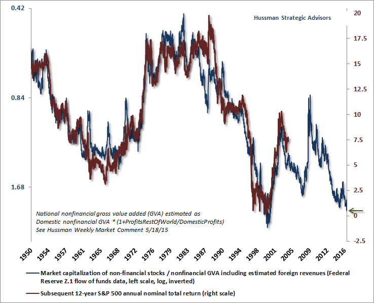
So?I?m wondering what the difference is between your algorithm for future returns and John Hussman?s algorithm for future returns. For history, up to the 10 year ago point, the two graphs look quite similar. However, for recent years within the 10-year span, the diverge quite substantially in absolute terms (although the shape of the ?curves? look quite similar). It appears that John?s algorithm takes into account the rise in the market during the 2005-2008 timeframe, and yours does not (as you stated, all else remaining the same, the higher the market is at any given point, the lower the expected future returns that can be for an economy). That results in shifting your expected future returns up by around 5% per year compared to his! That leads to remarkably different conclusions for the future.
Perhaps you have another blog post explaining your prediction algorithm that I have not seen. John has explained (and defended) his algorithm extensively. In absence of some explanation of the differences, I think that John?s is more credible at this point. See virtually any of his weekly posts for his chart, but the most recent should be at http://www.hussmanfunds.com/wmc/wmc161212e.png?(DJM: the article in question is here.)
I’d love to meet and talk with John Hussman. ?I have met some members of his small staff, and he lives about six miles from my house. ?(PS — Even more, I would like to meet @jesselivermore). ?The Baltimore CFA Society asked him to come speak to us a number of times, but we have been turned down.
Now, I’m not fully cognizant of everything he has written on the topic, but the particular method he is using now was first published on 5/18/2015. ?There is an article critiquing aspects of Dr. Hussman’s methods from Economic Philosopher. ?You can read EP for yourself, but I gain one significant thing from reading this — this isn’t Hussman’s first model on the topic. ?This means the current model has benefit of hindsight bias as he acted to modify the model to correct inadequacies. ?We sometimes call it a specification search. ?Try out a number of models and adjust until you get one that fits well. ?This doesn’t mean his model is wrong, but that the odds of it forecasting well in the future are lower because each model adjustment effectively relies on less data as the model gets “tuned” to eliminate past inaccuracies. ?Dr. Hussman has good reasons to adjust his models, because they have generally been too bearish, at least recently.
I don’t have much problem with his underlying theory, which looks like a modified version of Price-to-sales. ?It should be more comparable to the market cap to GDP model.
This model, to the best of my knowledge, has not been tweaked. ?It is still running on its first pass through the data. ?As such, I would give it more credibility.
There is another reason I would give it more credibility. ?You don’t have the same sort of tomfoolery going on now as was present during the dot-com bubble. ?There are some speculative enterprises today, yes, but they don’t make up as much of the total market capitalization.
All that said, this model does not tell you that the market can’t fall in 2017. ?It certainly could. ?But what it does tell you versus valuations in 1999-2000 is that if we do get a bear market, it likely wouldn’t be as severe, and would likely come back faster. ?This is not unique to this model, though. ?This is true for all of the models mentioned in this article.
Stock returns are probabilistic and mean-reverting (in a healthy economy with no war on your home soil, etc.). ?The returns for any given year are difficult to predict, and not tightly related to valuation, but the returns over a long period of time are easier to predict, and are affected by valuation more strongly. ?Why? ?The correction has to happen sometime, and the most likely year is next year when valuations are high, but the probability?of it happening in the 2017?are maybe 30-40%, not 80-100%.
If you’ve read me for a long time, you will know I almost always lean bearish. ?The objective is to become intelligent in the estimation of likely returns and odds. ?This model is just one of ones that I use, but I think it is the best one that I have. ?As such, if you look the model now, we should be Teddy Bears, not full-fledged Grizzlies.
That is my defense of the model for now. ?I am open to new data and interpretations, so once again feel free to leave comments.
[bctt tweet=”As such, if you look the model now, we should be Teddy Bears, not full-fledged Grizzly Bears.” username=”alephblog”]
Shiller trailing P/E chart has some value, but its been overused by perpetual bear marketers.
I think the high interest rates of the 70’s and 80’s are very far outside of historical interests rates. IMO current rates are far closer to historical average rates than those years. If rates were 10% above average rates for a significant chunk of P/E ratio chart then it really screws up the ability to use stock market valuations at that time.
Also post-WWII equity prices may not be relevant to today’s valuations. After WWII capital was very valuable as a lot of capital was destroyed during the war and had to be rebuilt. Plus we had 20 years of technological innovation that had not been implemented from the Great Depression. Now with decades of peace most of the highest return investments have already been used.
Equity valuations should be higher today than in the past. Until we hit some kind of technological breakthrough that supercharges growth.
I don’t know the correct P/E on the stock market. But a 6% equity return seems like a reasonable return if the US 30 year treasury is 3.2%. 300 bps of equity risks premium seems fair. If rates revert to mean with a 30 year in the 4-5% range then equities should yield a little more.
Look at the Doug Short link I posted. There is no correlation between CAPE and 10-year treasuries. Each bull and bear market shows distinct trend lines within them but they are not repeatable from secular bull/bear to another. So each bull and bear market has its own story line with its own internal trend lines that are different from other ones. So this market has a current story line but the participants could change it in a heartbeat which is probably what happens at key turning points. The Merkel/Livermore model above is focusing on what the participants are doing (Kahnemann-Taversky type of behavioral approach) instead of incantations using earnings, interest rates, and inflation.
So high CAPE tends to lead to lower 10-year returns than low CAPE, but there is a lot of scatter in that.
Does the large-scale issuance of debt (esp. by the Treasury) distort the calculations? Someone must hold that debt and it might make equity ownership look “small” in comparision.
Nick de Peyster
http://undervaluedstocks.info/
US Federal debt was bigger as a percentage of GDP in 1946 than today and that didn’t prevent the big post-war boom. However, financial sector, household, and non-financial business debt are much bigger today as a percentage of GDP than in 1946. That debt growth started in earnest after 1982, so it has been going on for a long time and is probably a major reason for the elevated CAPE and other valuation values over much of the past 20 years. Interestingly, interest rates and inflation rates are almost a perfect inverse of the growth of debt as a percentage of GDP over that period of time. The rise in income and wealth inequality in the US has also largely tracked the growth in debt over that time, so I suspect that the two are related but it may be just correlation and not causation. https://en.wikipedia.org/wiki/Financial_position_of_the_United_States#/media/File:Components-of-total-US-debt.jpg
https://en.wikipedia.org/wiki/Income_inequality_in_the_United_States#/media/File:U.S._Income_Shares_of_Top_1%25_and_0.1%25_1913-2013.png
BTW – the implicit guarantees that the US government and Fed have been providing the financial sector either for the financial company assets or the guaranteed home mortgages over the past eight years dwarf the issued Federal treasury debt to date. So the “debt ceiling” debate is really just a sideshow because the real potential financial system destabilizer is the financial system itself, not the Treasury debt issued to pay for government programs and military spending. So I am more concerned about the potential financial and economic impacts of deregulating the 100% of US GDP financial sector debt than adding some additional formal Treasury debt, especially given the low total tax per capita in the US compared to the rest of the developed world.
This series of posts have been very enlightening to me.
A couple of comments regarding the Shiller CAPE return predictions compared to the “prediction” in this post:
1. Many of the 7-10 year predictions I have seen based on CAPE are for “real” returns instead of nominal. If 2%-3% inflation is deducted from the 6.37%, the “real” return drops to the upper range of what often is predicted from the Shiller CAPE at current levels.
2. Ben Carlson did an interesting post a couple of days ago looking at nominal returns for past CAPE values. The 6.37% is about 4% above the mid-way point between the highest and lowest past 10 year returns for CAPE > 25 but is 3% less than the highest past return, so it is not an outlier. http://awealthofcommonsense.com/2016/12/expected-risk/
3. Doug Short’s site did an interesting analysis of past CAPE values in different interest rate and inflation environments. It is pretty clear that every bull market is on its own adventure with different relationships with those variables in each period. http://www.advisorperspectives.com/dshort/updates/2016/12/02/market-valuation-inflation-and-treasury-yields-clues-from-the-past
So the Merkel/Livermore model is probably as good as it gets for 10 year predictions for S&P 500 returns. However, Ben Carlson found that the volatility of the market was the same at all CAPE levels, so the best overall prediction of market action is JP Morgan’s “It will fluctuate”.